₊Method of Lagrange multipliers. Relative positioning of "repulsive" movable points on a circle
₊Modified version.
Let L be a circle of radius R around the point O: L:={x∈ℝ2: ||x||=R}. There is a set lP={p1, p2,...,pn} of n movable points and with each pi∈L,{(xi,yi)∈L: i = 1,...,n} -their coordinates. Let the points be "repulsive". f(x,y)= -sum of the distances from (x,y) to each point pi's. g(x,y)= - points (x,y)∈L.
Problem: use the method of Lagrange multipliers to find distribution of "repulsive" points on a circle corresponding to the maximum of their sum of mutual distances.
Step by step, all the points are iterated over each time until each point is at the Geometric medians(GM) points of the other n-1 points. We assume that the equilibrium - stationary state in system of n "charges" is reached if the sum of their mutual distances is maximal.
Critical points of maximum can be found using Lagrange multipliers as Λ(x,y,λ)=f(x,y)+λ*g(x,y) finding the critical points f(x,y) subject to: g(x,y)=0.
Iterative methods for optimization
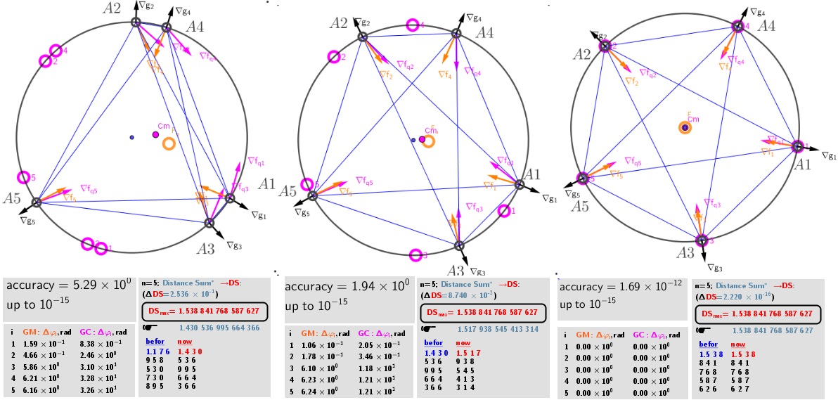
There is a system of equations: ∇f(x,y)= λ*∇g(x,y). A local optimum occurs when ∇f(x,y) and ∇g(x,y) are parallel, and so ∇f is some multiple of ∇g. Here, an iterative formula is used to find the points of the local maxima of the corresponding distance sum functions. Relationship between vectors of two consecutive iterations is defined in this case by - the new position of the s point: ∈L. All points are successively corrected (s = 1,2, ..., n) until the system of points comes to a stationary state. Finally, at the end of iterations they must match: ps=ps* for all s=1,2,...,n. The number of correction steps is carried out until the center of mass of n particles from lP (with a certain degree of accuracy) will not be in the center of the circle.
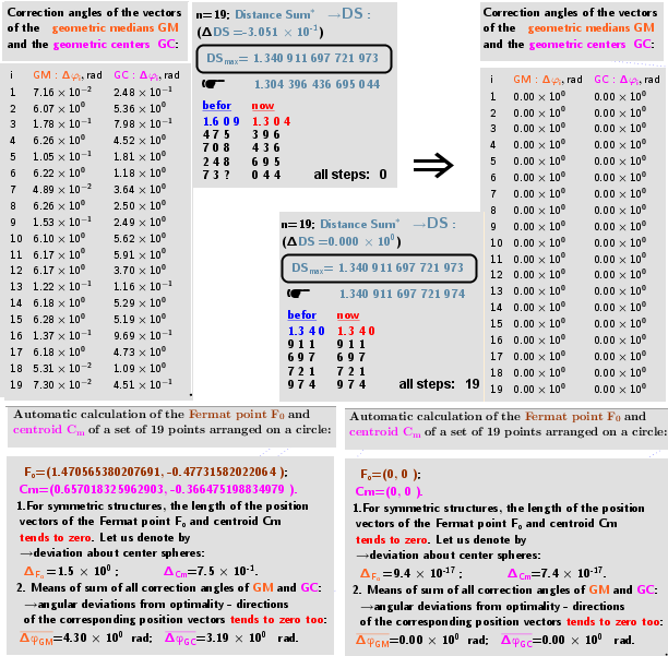
The solution of the above Lagrange problem means that in "equilibrium" for any point s from the set lP, their position vectors i. e. gradient ∇gs=/R -gradient of the magnitude of a position vector r, and the sums of the unit vectors of the other n-1 points: gradient ∇fs∼must be parallel, i.e. the angle Δφ between these two gradients vectors is multiple of π .
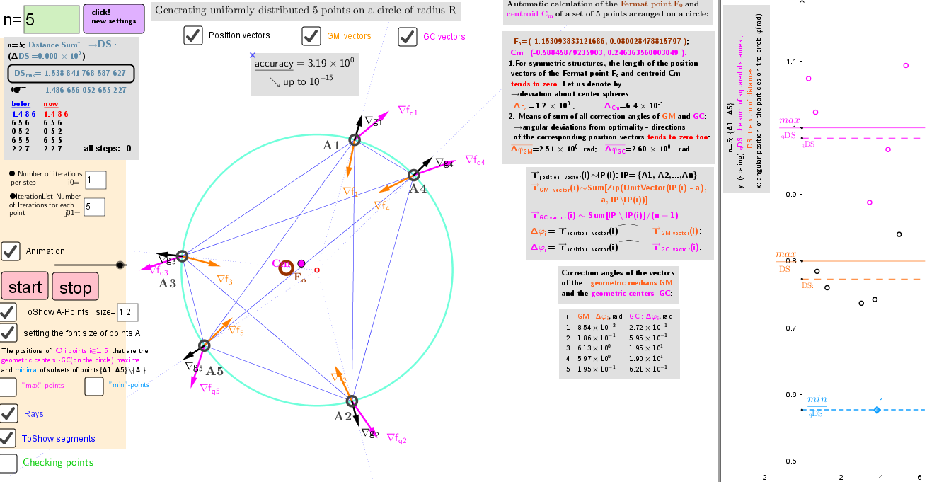
The gradients of the function sum of squares of their mutual distances are ∇fq s∼. The formulas for the position of the geometric centers of systems of n-1 points (on a circle) for the local maxima of the fq s -function of distances at each iteration step are determined each time by explicit formulas. Their coordinates, in contrast to Geometric Medians, have explicit formulas: GCmax= - R*UnitVector(Sum(lP)). This point and GCmin= R* UnitVector(Sum(lP))- two antipodal points on circle.
As it turns out, in the equilibrium position of the n -points system, each point is located both in the positions of the Geometric median(GM) and in the Geometric centers(GC) of the remaining points.
●Main iteration formula in applet: Execute(Join(Sequence(Sequence("SetValue(A"+i+",CopyFreeObject(Element[Last[IterationList((0,0)+R UnitVector(Sum[Zip[UnitVector(a-lP(r)),r,Sequence[n]\{"+i+"} ]]),a, {A"+i+"},j01)],1] ) )",i,1,n),ii,1,i0) ) ). IterationList -Number of Iterations for each point j01=5, i0 -number of iterations per step.
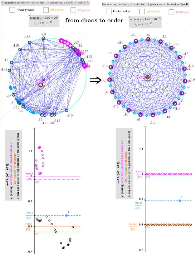
●An example of ordering points on a circle is a clear and illustrative of using the iterative method of finding geometric medians(GM) and geometric centers(GC) on a bounded domain for a system of points. Similar considerations were applied to finding a uniform distribution of points on a sphere.
Initial, intermediate and final -the "equilibrium" location of points on the circle as a result of an iterative procedure leading to the Maximum Distance Sum condition.