This applet describes tools that allow you to explore the properties of scalar and vector fields.
Applet design
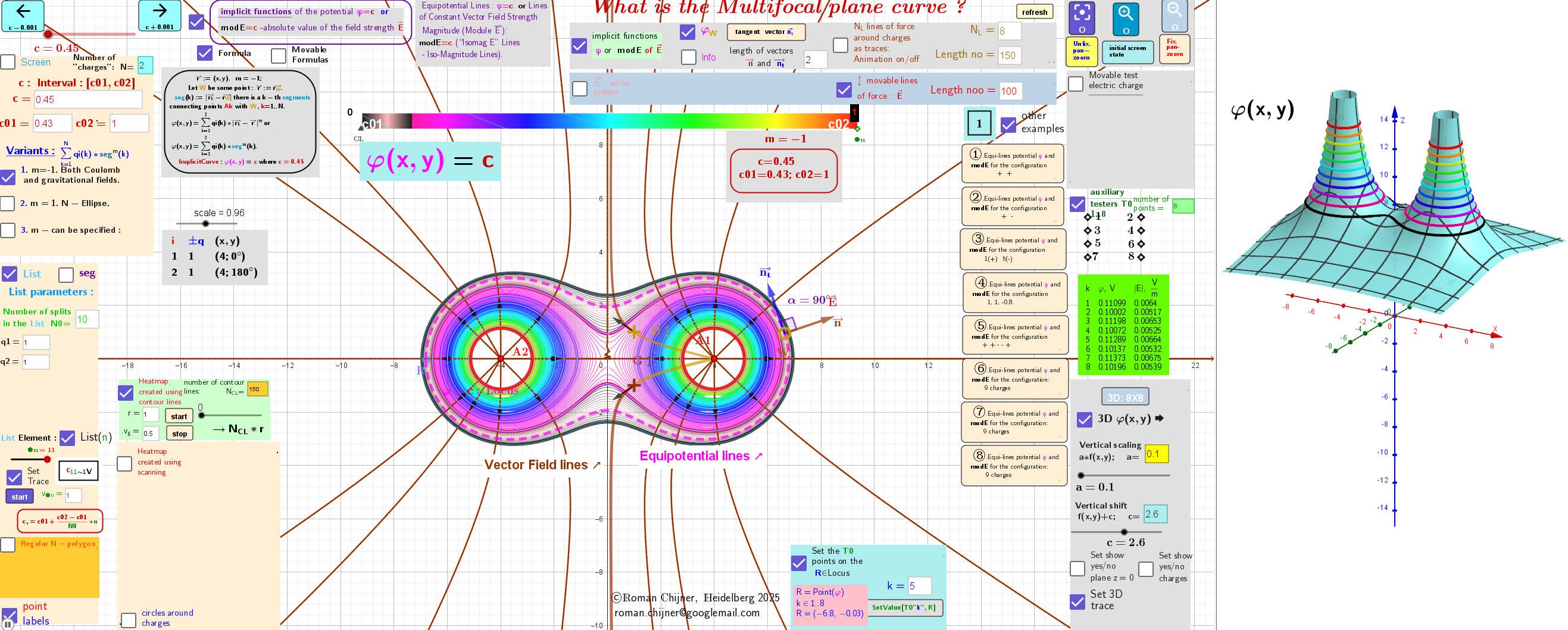
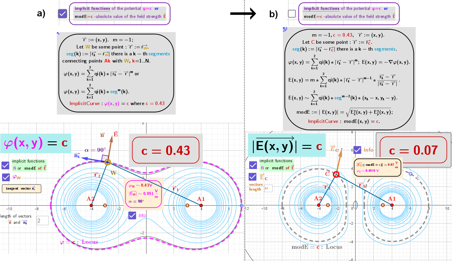
1.Finding a vector field from a scalar field of type φ(r)=Σqᵢ*|rᵢ –r|ᵐ, where m∈ℝ, by calculating its gradient: E = - ∇ φ.
There are two different ways of representing loci for the system of "charges":
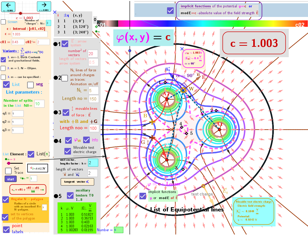
a) equipotential lines, φ =c, and
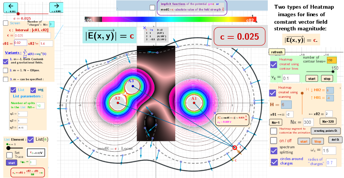
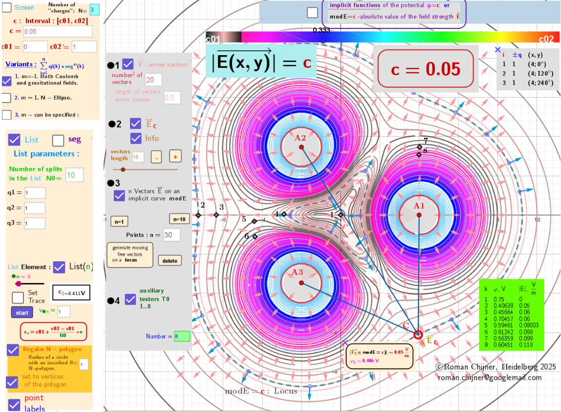
b) lines of constant magnitudes of the corresponding conservative vector field, modE = c.
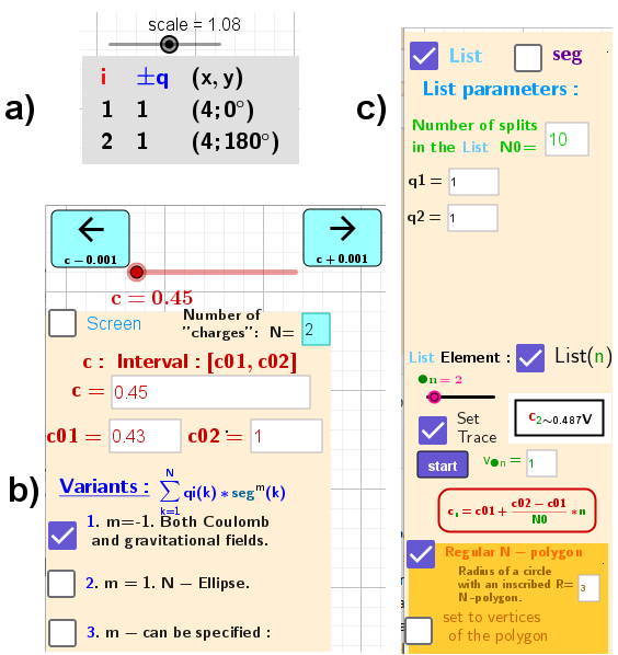
2. Particular known cases of fields and their parameters.
For the system A1, A2,..
a) of N (maximum 9) point "charges"
b) the lower boundaryc01 and the upper boundaryc02 are found (by selection) for a constant value c, so that the loci
b) from the List are adjust for the corresponding fields. The boundaries c01 and c02 are found separately for the representation of equipotential fields φ=c, as well as for the lines of constant values of the vector field modE=c.
3. The electric field and equipotential lines for three equal charges at the vertices of an equilateral triangle.
Instructions.
Methods of visualization of equipotential lines, direction and magnitude of a vector fields
●1. Using a variable-length array, you can represent the direction of a vector field over the entire observation field using arrows.
●2. Vector field lines of force are drawn around each charge. They start at some charges and end at opposite charges or at infinity.
●3 By installing a movable point +B and +G at any observation point, the vector field line of force passing through it is represented.
●4. At the locusφ=c, there is a movable point W and with its help you can check the orthogonality of the equipotential lines and field lines of the vector field. The same can be done using a movable test charge.
●5. Using a set of movable test charges T0 (up to 8), you can also test the potential and magnitude of the field, the values of which are summarized in the table.
4. Lines of constant vector field strength magnitude are closed confocal curves, the foci of which are located at the charges.
Lines of constant vector field strength magnitude, often called level curves or isolines, are curves in a vector field where the magnitude of the vector field is constant: modE=c “Isomag E” Lines - Iso-Magnitude Lines.
In simpler terms, they are curves where the "strength" of the field is the same at every point along the curve. They are closed confocal curves, the foci of which are located at the charges. The magnitude of the vector field strength is the same at all loci, but the directions of the field vectors differ. The circulation of the field vector along these closed curves is zero because the field is conservative. Therefore, if the segments of the curve are the same, the infinite sum of the cosines of the angles between the field vectors and the vectors of the sections of this curve is also zero.
5. Two Types of Heatmap images for Equipotential lines.
The Heatmap, created by scanning outside parameter c interval, draws black and white curves.
6. Two Types of Heatmap images for lines of constant vector field strength magnitude.
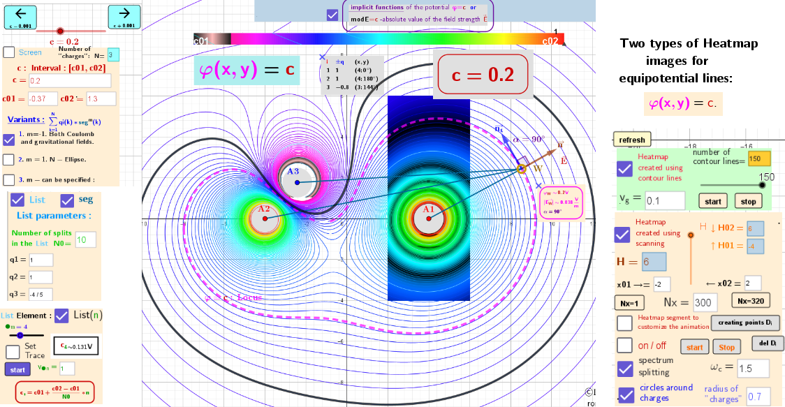
![[size=85] The Heatmap, created by scanning outside parameter [color=#980000]c interval[/color], draws black and white curves.[/size]](https://www.geogebra.org/resource/vt3dzjwy/h85NmqmtUMcpmHYC/material-vt3dzjwy.png)