Deterministic model
We have already worked our way through the
first two steps, so it remains to implement
the GeoGebra applet. In this model we quickly create two sliders in GeoGebra, one for
the key interest rate p and the other for the exchange rate er. In the spreadsheet-view
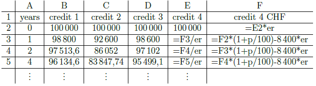
one calculates the yearly debt level for the four credits by using the recurrence relation
(1). For Example in cell B1 one
nds the formula "=B2*(1+p/100)-8 400", analogous
calculations for credit 2 (pay attention to the
rst two periods!) and credit 3 (use if-
statements!). The calculations of credit 4, see table 1, lead to the same yearly debt levels
as for credit 1.
Table 1
We follow the idea of Heugl and create a list of points for every credit (see [3], p. 76).
The result is a nice visualization of the yearly debt levels of each credit. Different point
styles enable easy distinguishing between the four credits.
Figure 2.1
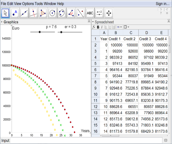
Figure 2.2
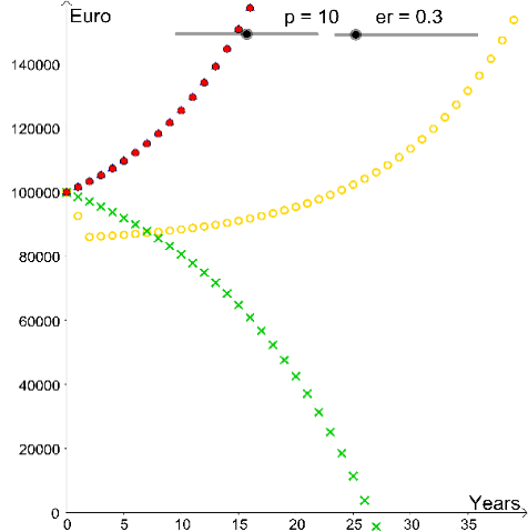
In school a stage of experiments might be of advantage, like manipulating slider bars
and observing its outcomes. In case of less experienced pupils the teacher should prepare
guiding questions, e.g. "What will happen, if the value of the key interest rate in-
creases/decreases?" or "At which values is credit 1 better than credit 2?" These heuristic
observations can be collected and shared in class.
Afterwards there is an opportunity to justify some of these
findings by using mathe-
matical argumentations. In this deterministic model one gets for every value of the key
interest rate p one best credit or for some values p two best credits, see below.
One gets such values by pairwise comparing the credits. For example one obtains 1.477
by using the equation (2) of credit 1 and 2 (slightly modified) and set Sn = 0. We express
the number of years n explicitly. In case of credit 1 we get per CAS (for convenience we
set q := 1 + p/100 ):
We equal the two terms of the equations (3) and (4) and solve the resulting equation for
the variable q. Finally, we obtain q = 1.01477 and therefore p = 1.477.
In a validation of this model one will recognize some of its wrong results. It is impossible
that the yearly debt level of the foreign currency loan equals the yearly debt level of
credit 1. Empirical investigations like reading newspaper reveal this mistake in the model
above. Foreign currency loans have a bad press, actually in Austria they are forbidden
for hypothecary credits.