The Simple Pendulum
The pendulum is a common system when you consider all the hanging objects in the world that can be made to swing. Most of the real pendulums (more correct than pendula as a plural) are not quite ideal and would require more considerations than just mass.
The ideal (also called simple) pendulum, which we will discuss exclusively in this section, is assumed to have all of its mass concentrated at a point, and there is no mass associated with the support string or rod. Further, a simple pendulum is assumed unaffected by drag or any friction. Of course real pendulums experience tiny bits of friction from things like air drag, but assuming that friction is negligible is a good place to start. In the case of such an ideal pendulum, the only force that causes it to swing is the gravitational force.
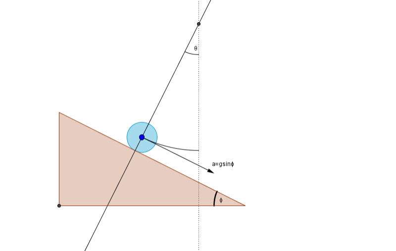
The force of gravity does not cause it to accelerate at the rate of free fall since only a small component of gravity acts along the direction of the swing. In this sense it is identical to a friction-less block on an incline. The component of the gravitational force down the incline is , where is the angle of the incline. If you imagine the pendulum to not be supported by tension in a string or rod, but rather to be sliding inside a spherically shaped bowl and supported by a normal force, then you realize that the physics is just like a friction-less block on an incline, and that the angle of the incline represents the swing angle.
To see what I mean about the incline versus the swing angle, notice that in the diagram below, that Imagine that the blue ball is the pendulum bob, and notice that its swing angle with respect to the vertical line is the same as the slope of an incline tangent to its path at that point in its swing. This means that the acceleration along the arc will just be .
Solving the Pendulum Equation
A mass on the end of a rod is subject to only that force discussed above. In this context it is called a restoring force. It is called a restoring force since it tries to restore the pendulum to its equilibrium location in which it hangs vertically. As mentioned, the restoring force is the same force that pulls a block down an incline of slope , but in the case of the pendulum, moment by moment the angle is changing. The minus sign needs to be there because the force is opposite the direction of increasing angle. It is important to recognize that the pendulum's restoring force is a non-linear function. It is not proportional to the swing angle, which would make it linear, but to the sine of that angle. This non-linear restoring force means that the resulting motion is not simple harmonic. As such, we should expect that the swing angle will affect the period of the pendulum and the plot of the angle versus time will not be sinusoidal - even if your eye might argue that it is. In reality it's just a very good counterfeit of sinusoidal motion.
Mathematically, we can use the restoring force as the net force in Newtons 2nd law, just as we did with the mass on a spring, and arrive at the equation .
In order to find the motion of the pendulum, we need to turn this into a differential equation just as we did for the mass and spring system. Using the equation for arc length , we can take two derivatives with respect to time, and while assuming 'r' is constant, arrive at . As the pendulum swings, it traces out an arc segment, so this acceleration is tangent to the arc along which it travels. This is not centripetal acceleration.
Next, we substitute this acceleration into our equation for the pendulum above and get . Cleaning up the expression by putting both terms on the same side and dividing out the radius (which represents the length of rod or string) gives us
This equation has no solution for in terms of analytic functions. This means that there is no way to solve for the exact motion of the pendulum using math on pen and paper. In order to be able to say anything useful about the pendulum while doing math with paper and pen, and to be able to write an expression for period or angular frequency, we need to approximate the sine function in the differential equation for small angles. This way we can continue on paper rather than immediately turning to numerical methods to solve the equation. But be forewarned that doing so leads to results that are only approximate, and are only valid for small swing angles.
It is the sine function that makes this differential equation unsolvable. Therefore we need a simplification of it. We will replace the sine function with a Taylor series approximation for sin x.
An aside: It is possible to solve this pendulum differential equation with advanced series solutions, but these solutions have an infinite number of terms, and in that sense aren't exact solutions in terms of a finite set of common analytic functions. In an advanced class on differential equations you may one day learn about such solutions.
Taylor Series
A Taylor series is a series of polynomial functions used to approximate some other function such as a sine function in the pendulum equation above. The more terms in the series, the more accurate the approximation. Taylor polynomials are very commonly used in physics and engineering to simplify expressions that are otherwise not able to be solved analytically. Our pendulum differential equation is a good example of this. In cases where the argument to a function does not tend to stray far from a particular value (like the angle of the pendulum's swing being small), the Taylor series approximation is a very accurate substitute for the actual function. Furthermore, while a Taylor series can in principle have an infinite number of terms, usually only the first non-constant term in the expression is retained. Keeping more terms almost always results in a differential equation that is still impossible to solve, but there are exceptions to this.
The mathematical definition of a Taylor series approximation of order N for a function approximated at x=a is:
The primes (') are to be understood to represent derivatives so that is the ith derivative of F. If you look at the terms, we can interpret the Taylor series as a series of terms, the first of which matches the value of the actual function, the second of which matches the slope of the actual function, the third of which matches the concavity or curvature of the actual function, the fourth of which matches the rate of change of concavity of the actual function, and so on.
The value of 'a' is chosen as that value of x where you want the series approximation to best match the original function. In the case of the pendulum, 'x' is really our swing angle , and we want it to do its best around equilibrium where the value is zero. So we want a=0 in the present example. In spite of this, I made the interactive graphic below so that you can change the value of 'a'. The highest polynomial power in the series (N) is also adjustable in the graphic below.
Taylor Series Approximation of sin(x)
Using the first order approximation from the Taylor series tells us that with x in radians. It can be seen in the plot above of the Taylor expansion of sin(x) that until the swing angle takes on a value of around 0.5 rad or greater, the functions are very close in value. You can drag the slider for N, and see what higher order Taylor series approximations for sin(x) look like, and by changing 'a' you can center the approximation at another value rather than zero. Notice that when we choose x=0, that only odd-powered terms are non-zero, but that when x is non-zero, all terms, odd or even, survive.
If we make the substitution , the pendulum equation becomes identical in form to that of the mass and the spring system which led to SHM, except that the constants are different. The equation becomes
.
A general solution to this equation is identical in form to the solution for the mass-spring system, and is . Keep in mind that you have some freedom in choosing the functional form. Two alternatives that are mathematically equivalent are: You may choose whichever seems to fit the problem best. While it will look different if you choose a different equation, the predicted swing angle, velocity, acceleration will be the same regardless. As in the spring/mass system, knowing something about the initial conditions will allow us to specify the unknown constants - either A and B, or A and . For instance, knowing that the pendulum starts from rest at amplitude is enough information to determine the constants. Here is the solution in written in each functional form. or Because we see that by evaluating at time t=0s in either solution tells us that A=, and the value of in the second solution is likewise zero. So either one amounts to the equation . For the pendulum, the angular frequency for small swing angles is given by where r is the radius of the arc along which the pendulum swings (length of the string from which a mass hangs). Notice that angular frequency has no dependence on the mass of the pendulum, only on the arc radius and the gravitational constant g. Since we see that ordinary frequency and the period of the pendulum (time to swing to and fro) are also independent of mass and only depend on the gravitational field and the radius of the arc along which it swings.Actual Pendulum versus the Approximate Solution
Since we had to use a small angle approximation to solve the differential equation of motion for a pendulum, it's worth wondering how good the solution is. How close is that approximated solution to the actual pendulum's motion? I have used GeoGebra to calculate the actual pendulum's motion using numerical methods and plotted it compared with the approximate (small-angle) solution below. The orange plot is the solution according to the small angle approximation that we used. The black dashed plot is the numerical solution of the actual pendulum equation. The red plot is a cosine function that best fits the actual motion so that you can compare the shape of a cosine to the actual motion.
It is clear that at small angles the curves of the actual motion (black) and the red cosine wave have a very similar shape. Notice, however, that even with relatively small initial angles (which you have control of) that the period of the pendulum changes as compared with the small angle solution. When the wave gets longer we should understand that there is an increase in the period (T) of the swing. At an initial angle of the period is increased by roughly 50%, but even at smaller angles it's noticeable. Can you understand why the plot of the actual motion (black) becomes completely flat an an initial angle of ?